Sample Problems > Usage > Plotting > plot_on

{ PLOT_ON_GRID.PDE

This is a variation of BENTBAR.PDE that makes use of

the capability to plot contours on a deformed grid.

The syntax of the plot command is

CONTOUR(data) ON GRID(Xposition,Yposition)

}

title "Contour plots on a deformed grid"

select

cubic { Use Cubic Basis }

variables

U { X-displacement }

V { Y-displacement }

definitions

L = 1 { Bar length }

hL = L/2

W = 0.1 { Bar thickness }

hW = W/2

eps = 0.01*L

I = 2*hW^3/3 { Moment of inertia }

nu = 0.3 { Poisson's Ratio }

E = 2.0e11 { Young's Modulus for Steel (N/M^2) }

{ plane stress coefficients }

G = E/(1-nu^2)

C11 = G

C12 = G*nu

C22 = G

C33 = G*(1-nu)/2

amplitude=GLOBALMAX(abs(v)) { for grid-plot scaling }

mag=1/amplitude

force = -250 { total loading force in Newtons (~10 pound force) }

dist = 0.5*force*(hW^2-y^2)/I { Distributed load }

Sx = (C11*dx(U) + C12*dy(V)) { Stresses }

Sy = (C12*dx(U) + C22*dy(V))

Txy = C33*(dy(U) + dx(V))

{ Timoshenko's analytic solution: }

Vexact = (force/(6*E*I))*((L-x)^2*(2*L+x) + 3*nu*x*y^2)

Uexact = (force/(6*E*I))*(3*y*(L^2-x^2) +(2+nu)*y^3 -6*(1+nu)*hW^2*y)

Sxexact = -force*x*y/I

Txyexact = -0.5*force*(hW^2-y^2)/I

initial values

U = 0

V = 0

equations { the displacement equations }

U: dx(Sx) + dy(Txy) = 0

V: dx(Txy) + dy(Sy) = 0

boundaries

region 1

start (0,-hW)

load(U)=0 { free boundary on bottom, no normal stress }

load(V)=0

line to (L,-hW)

value(U) = Uexact { clamp the right end }

mesh_spacing=hW/10

line to (L,0) point value(V) = 0

line to (L,hW)

load(U)=0 { free boundary on top, no normal stress }

load(V)=0

mesh_spacing=10

line to (0,hW)

load(U) = 0

load(V) = dist { apply distributed load to Y-displacement equation }

line to close

plots

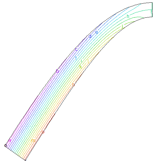
grid(x+mag*U,y+mag*V) as "deformation" { show final deformed grid }

! STANDARD PLOTS:

contour(U) as "Contour on Static Grid"

surface(U) as "Surface on Static Grid"

! THE DEFORMED PLOTS:

contour(U) on grid(x+mag*U,y+mag*V) as "Contour on Deformed Grid"

surface(U) on grid(x+mag*U,y+mag*V) as "Surface on Deformed Grid"

end

plot_on_grid

plot_on_grid