Sample Problems > Usage > Import

{ SPLINETABLE.PDE

This example solves the same system as TABLE.PDE, using a Spline interpretation of the

data in the table file 'TABLE.TBL'.

The file format is the same for TABLE or SPLINE TABLE input.

The SPLINE TABLE operator can be used to build spline tables of one or two dimensions.

The resulting interpolation is third order in the coordinates, with continuous values

and derivatives. First or second derivatives of the interpolated function may be computed.

Here the table is used as source and diffusivity in a fictitious heat equation, merely to

show the use of the table variable.

The SAVE function is used to construct a Finite Element interpolation of the data from the

spline table, for comparison of derivatives. Cubic FEM basis is used so that the second

derivative is meaningful.

}

title 'Spline Table Input Test'

select

regrid=off

variables

definitions

alpha = spline table('table.tbl') ! construct spline fit of table:

beta = 1/alpha

femalpha = save(alpha) ! save a FEM interpolation of table:

equations

U: div(alpha*grad(u)) + beta = 0

boundaries

region 1

start(0,10)

value(u) = 0

line to (0,0) to (10,0) to (10,10) to close

monitors

contour(u)

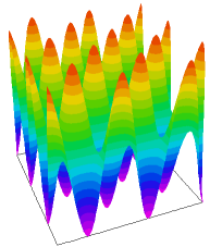
plots

grid(x,y)

contour(alpha) as 'table'

contour(dx(alpha)) as 'dx(table)'

contour(dy(alpha)) as 'dy(table)'

vector(grad(alpha)) as 'grad(table)'

surface(alpha) as 'table'

contour(dxx(alpha)) as 'dxx(table)'

contour(dxy(alpha)) as 'dxy(table)'

contour(dyy(alpha)) as 'dyy(table)'

contour(dxx(alpha)+dyy(alpha)) as "Table Curvature"

contour(div(grad(femalpha))) as "FEM Curvature"

surface(beta) as "table reciprocal"

contour(u) as "temperature solution"

surface(u) as "temperature solution"

end

splinetable