<< Click to Display Table of Contents >> Navigation:  User Guide > Complex Variables > The Time-Sinusoidal Heat

Suppose we wish to discover the time-dependent behavior of our example Cartesian blob due to the application of a time-sinusoidal applied temperature.

The time-dependent heat equation is Div(K*Grad(Phi)) = Cp*dt(Phi)

If we assume that the boundary values and solutions can be represented as

Phi(x,y,t) = Aphi(x,y)*exp(i*omega*t)

Substituting in the heat equation and dividing out the exponential term, we are left with a complex equation

Div(K*Grad(Aphi)) - Complex(0,1)*omega*Cp*Aphi = 0

The time-varying temperature Phi can be recovered from the complex Aphi simply by multiplying by the appropriate time exponential and taking the real part of the result.

Assuming for simplicity that omega=1 and Cp=1, the modified script becomes:

TITLE 'Heat flow around an Insulating blob'

VARIABLES

APhi = Complex(APhir,APhii)        { the complex temperature amplitude }

DEFINITIONS

K = 1                { default conductivity }

R = 0.5                { blob radius }

EQUATIONS

APhi: Div(-k*grad(APhi)) - Complex(0,1)*APhi = 0

BOUNDARIES

REGION 1 'box'

START(-1,-1)

VALUE(APhi)=Complex(0,0)        LINE TO (1,-1)

NATURAL(APhi)=Complex(0,0)        LINE TO (1,1)

VALUE(APhi)=Complex(1,0)        LINE TO (-1,1)

NATURAL(APhi)=Complex(0,0)        LINE TO CLOSE

REGION 2 'blob'        { the embedded blob }

k = 0.01        { change K for prettier pictures }

START 'ring' (R,0)

ARC(CENTER=0,0) ANGLE=360 TO CLOSE

PLOTS

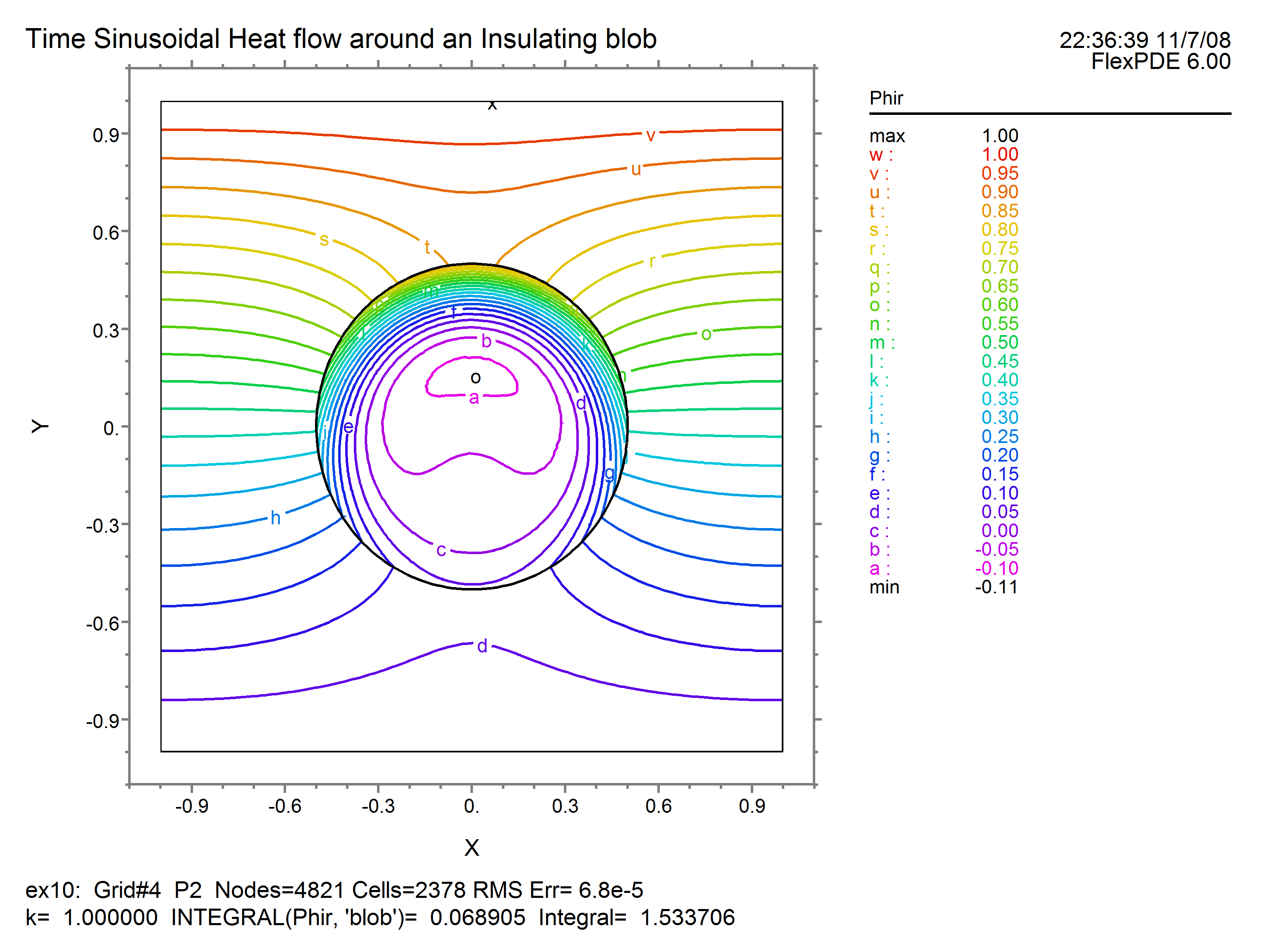
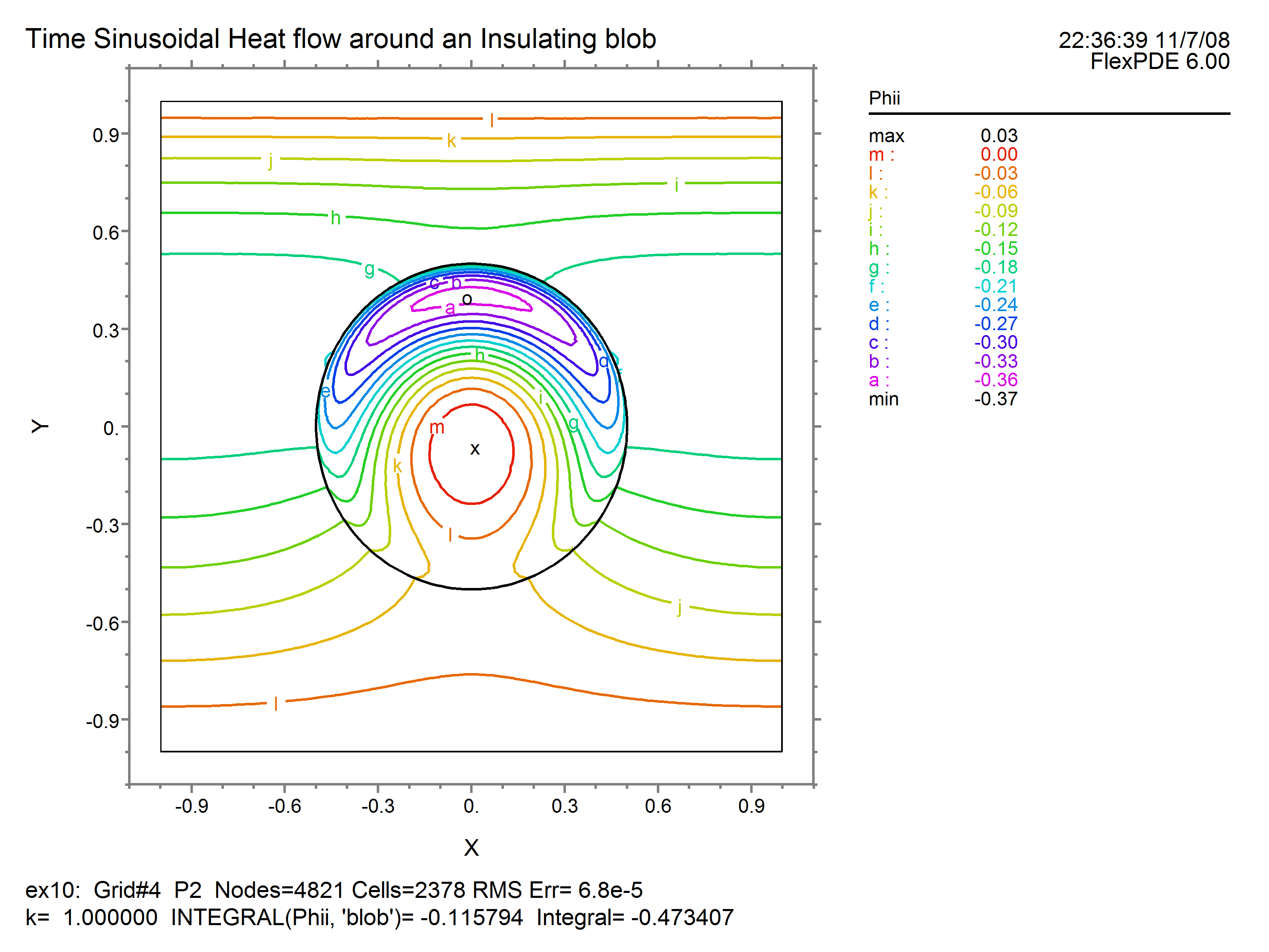
CONTOUR(APhir) CONTOUR(APhii)

VECTOR(-k*grad(APhir))

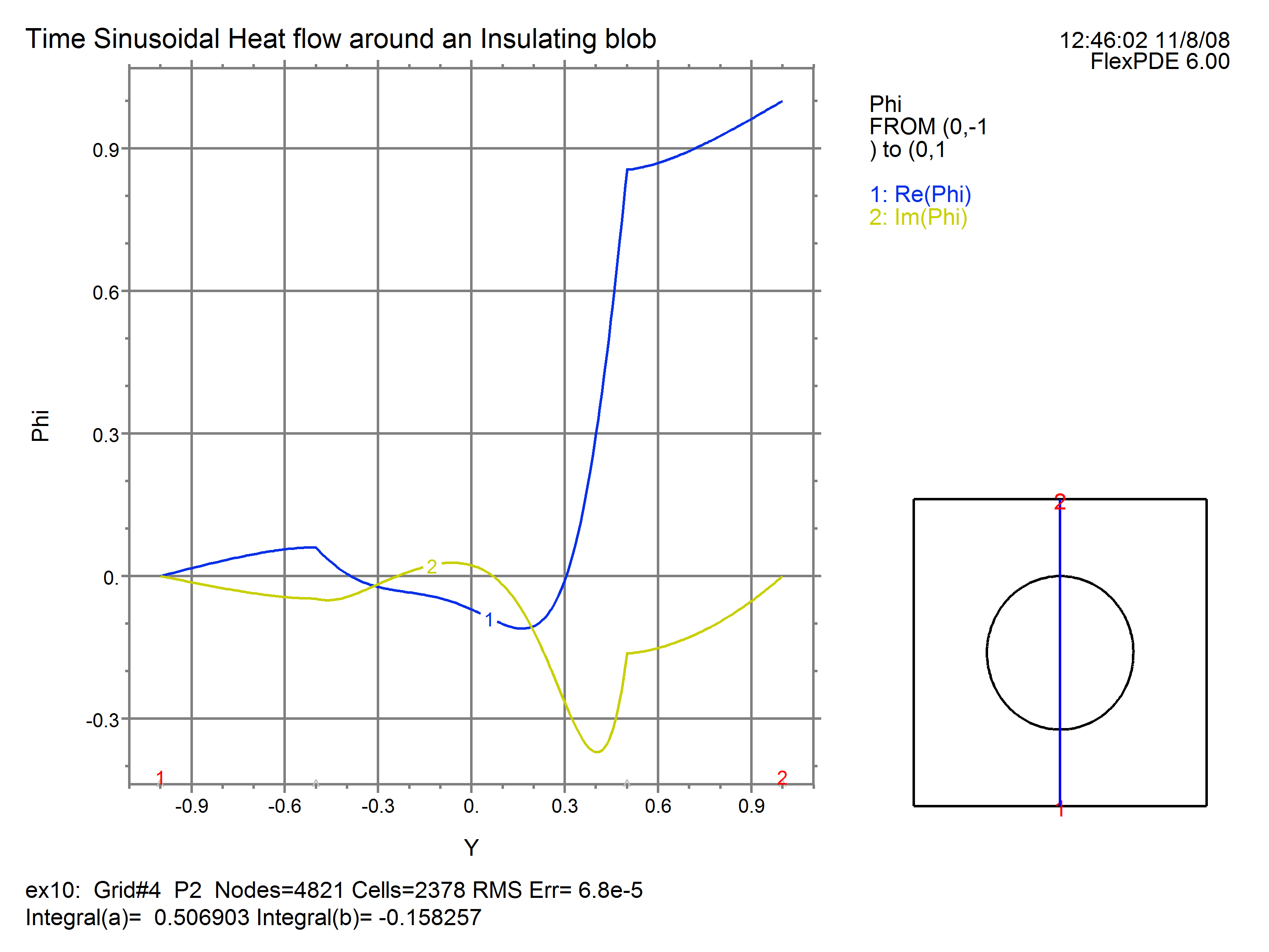
ELEVATION(APhi) FROM (0,-1) to (0,1)

ELEVATION(Normal(-k*grad(APhir))) ON 'ring'

END

 

Running this script produces the following results for the real and imaginary components:

 

 

 

The ELEVATION trace through the center shows: