<< Click to Display Table of Contents >> Navigation:  User Guide > Using FlexPDE in Three-Dimensional Problems > Shaped Layer Interfaces

We have stated that the layer interfaces need not be planar.  But FlexPDE makes some assumptions about the layer interfaces, which places some restrictions on the possible figures.

 

•Figures must maintain an extruded shape, with sidewalls and layer interfaces (the sidewalls cannot grow or shrink)

•Layer interface surfaces must be continuous across region boundaries.  If a surface has a vertical jump, it must be divided into layers, with a region interface at the jump boundary and a layer spanning the jump. (Not this:   but this:  )

•Layer interface surfaces may merge, but may not invert.  Use a MAX or MIN function in the surface definition to block inversion.

Using these rules, we can convert the canister of our example into a sphere by placing spherical caps on the cylinder.  

The equation of a spherical end cap is

Z = Zcenter + sqrt( R^2 – x^2 – y^2)

Or,

Z = Ztop – R + sqrt(R^2 – x^2 – y^2)

•To avoid grazing contact of this new sphere with the top and bottom of our former box, we will extend the extrusion from –1 to 1.

•To avoid arithmetic errors, we will prevent negative arguments of the sqrt.

 

Our modified script now looks like this:

TITLE 'Heat flow around an Insulating Sphere'

COORDINATES

Cartesian3

VARIABLES

Phi                { the temperature }

DEFINITIONS

K = 1                { default conductivity }

R = 0.5        { sphere radius }

{ shape of hemispherical cap: }

Zsphere = sqrt(max(R^2-x^2-y^2,0))        

EQUATIONS

Div(-k*grad(phi)) = 0        

EXTRUSION

SURFACE 'Bottom'  z=-1

LAYER 'underneath'

SURFACE 'Sphere Bottom'  z = -max(Zsphere,0)

LAYER 'Can'

SURFACE 'Sphere Top'  z = max(Zsphere,0)

LAYER 'above'

SURFACE 'Top'        z=1

BOUNDARIES

REGION 1 'box'

START(-1,-1)

VALUE(Phi)=0        LINE TO (1,-1)

NATURAL(Phi)=0        LINE TO (1,1)

VALUE(Phi)=1        LINE TO (-1,1)

NATURAL(Phi)=0        LINE TO CLOSE

LIMITED REGION 2        'blob'        { the embedded blob }

LAYER 2 K = 0.001

START 'ring' (RSphere,0)

ARC(CENTER=0,0) ANGLE=360

TO CLOSE

PLOTS

GRID(y,z) on x=0

CONTOUR(Phi) on x=0

VECTOR(-k*grad(Phi)) on x=0

ELEVATION(Phi) FROM (0,-1,0) to (0,1,0)

END

 

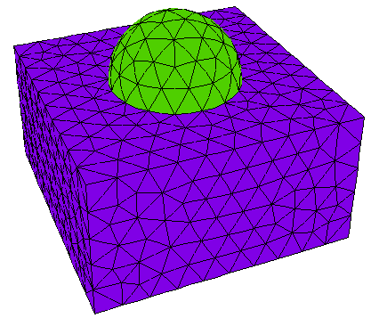
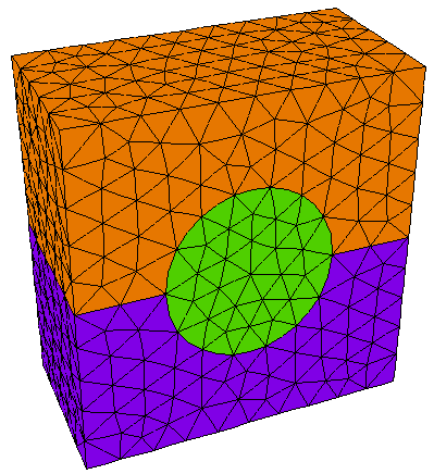
Cut-away and cross-section images of the LAYER x REGION compartment structure of this layout looks like this:

 

   

 

 

The contour plot looks like this:

 

 

 

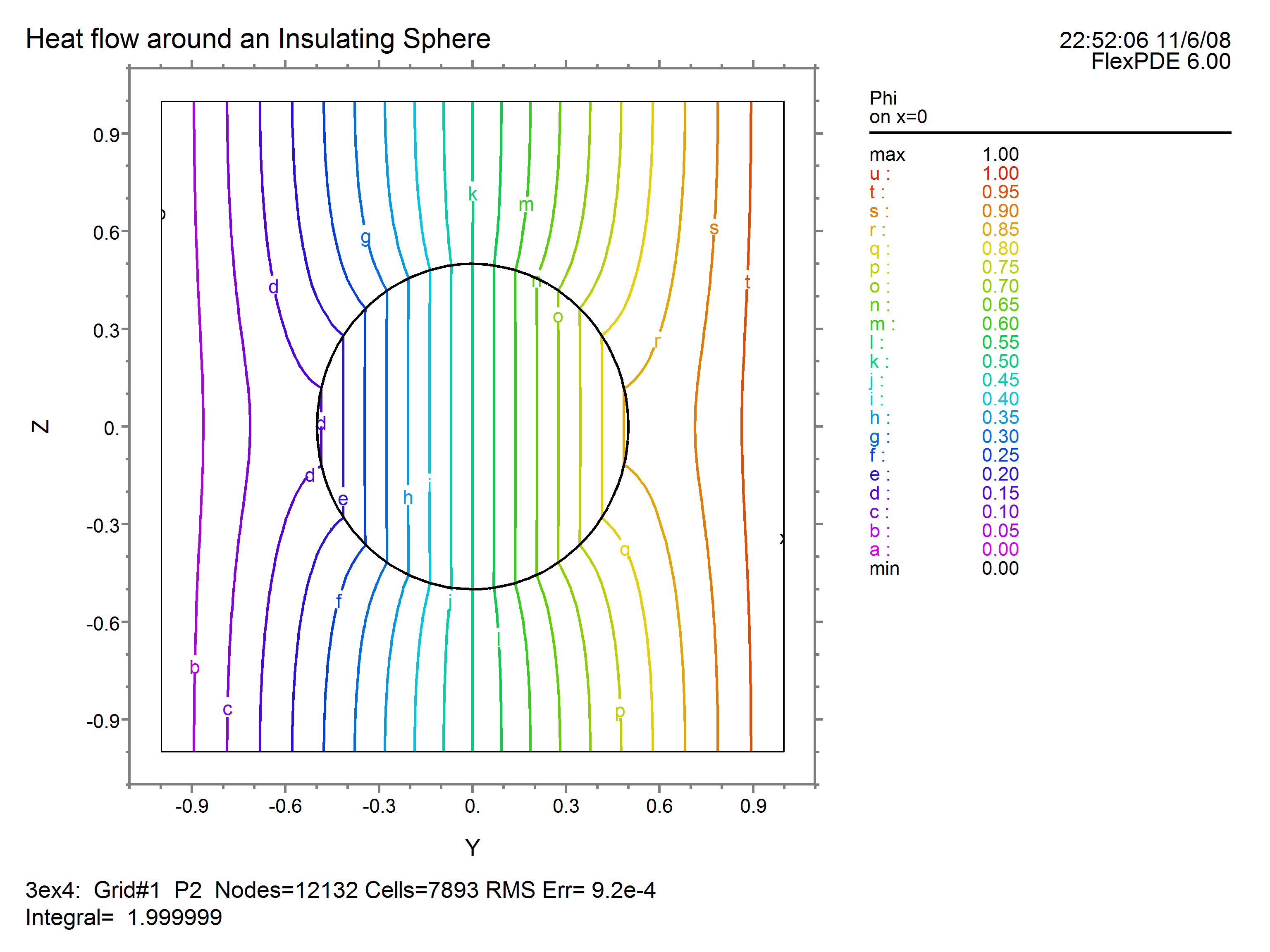
Notice that because of the symmetry of the 3D figure, this plot looks like a rotation of the 2D contour plot in "Putting It All Together".