Sample Problems > Applications > Heatflow > radiation

{ RADIATION_FLOW.PDE

This problem demonstrates the use of FlexPDE

in the solution of problems in radiative transfer.

Briefly summarized, we solve a Poisson equation

for the radiation energy density, assuming that

at every point in the domain the local

temperature has come into equilibrium with the

impinging radiation field.

We further assume that the spectral character-

istics of the radiation field are adequately

described by three average cross-sections:

the emission average, or "Planck Mean", sigmap;

the absorption average, sigmaa; and the transport

average, or "Rosseland Mean-Free-Path", lambda.

These averages may, of course, differ in various

regions, but they must be estimated by facilities

outside the scope of FlexPDE.

And finally, we assume that the radiation field

is sufficiently isotropic that Fick's Law, that

the flux is proportional to the gradient of the

energy density, is valid.

The problems shows a hot slab radiating across an

air gap and heating a distant dense slab.

}

title 'Radiative Transfer'

variables

erad { Radiation Energy Density }

definitions

source { declare the parameters, values will follow }

lambdar { Rosseland Mean Free Path }

sigmap { Planck Mean Emission cross-section }

sigmaa { absorption average cross-section }

beta = 1/3 { Fick's Law proportionality factor }

materials

'air' : source=0 sigmap=2 sigmaa=1 lambdar=10

'hot slab' : source=100 sigmap=10 sigmaa=10 lambdar=1

'dense slab' : source=0 sigmap=10 sigmaa=10 lambdar=1

equations { The radiation flow equation: }

erad : div(beta*lambdar*grad(erad)) + source = 0

boundaries

region 1 { the bounding region is tenuous }

use material 'air'

start(0,0)

natural(erad)=0 { along the bottom, a zero-flux symmetry plane }

line to (1,0)

natural(erad)=-erad { right and top, radiation flows out }

line to (1,1) to (0,1)

natural(erad)=0 { Symmetry plane on left }

line to close

region 2 { this region has a source and large cross-section }

use material 'hot slab'

start(0,0)

line to (0.1,0) to (0.1,0.5) to (0,0.5) to close

region 3 { this opaque region is driven by radiation }

use material 'dense slab'

start(0.7,0)

line to (0.8,0) to (0.8,0.3) to (0.7,0.3) to close

monitors

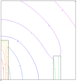
contour(erad)

plots

contour(erad) as 'Radiation Energy'

surface(erad) as 'Radiation Energy'

vector(-beta*lambdar*grad(erad)) as 'Radiation Flux'

{ the temperature can be calculated from the assumption of equilibrium: }

contour(sqrt(sqrt(erad*sigmaa/sigmap))) as 'Temperature'

surface(sqrt(sqrt(erad*sigmaa/sigmap))) as 'Temperature'

end

radiation_flow

radiation_flow