Sample Problems > Applications > Heatflow > axisymmetric

{ AXISYMMETRIC_HEAT.PDE

This example demonstrates axi-symmetric

heatflow.

The heat flow equation in any coordinate

system is

div(K*grad(T)) + Source = 0.

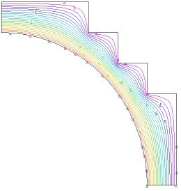
The following problem is taken from

Zienkiewicz, "The Finite Element Method

in Engineering Science", p. 306 (where

the solution is plotted, but no dimensions

are given). It describes the flow of heat

in a spherical vessel.

The outer boundary is held at Temp=0,

while the inner boundary is held at Temp=100.

}

title "Axi-symmetric Heatflow "

coordinates

ycylinder("R","Z") { select a cylindrical coordinate system, with

the rotational axis along the "Y" direction

and the coordinates named "R" and "Z" }

variables

Temp { Define Temp as the system variable }

definitions

K = 1 { define the conductivity }

source = 0 { define the source (this problem doesn't have one) }

Initial values

Temp = 0 { unimportant in linear steady-state problems }

equations { define the heatflow equation: }

Temp : div(K*grad(Temp)) + Source = 0

boundaries { define the problem domain }

Region 1 { ... only one region }

start(5,0)

natural(Temp)=0 { define the bottom symmetry boundary condition }

line to (6,0)

value(Temp)=0 { fixed Temp=0 in outer boundary }

line to (6,3) { walk the funny stair-step outer boundary }

to (5,3)

to (5,4)

to (4,4)

to (4,5)

to (3,5)

to (3,6)

to (0,6)

natural(Temp)= 0 { define the left symmetry boundary }

line to (0,5)

value(Temp)=100 { define the fixed inner temperature }

arc( center=0,0) to close { walk an arc to the starting point }

monitors

contour(Temp) { show contour plots of solution in progress }

plots { write these hardcopy files at completion }

contour(Temp) { show solution }

surface(Temp)

vector(-2*pi*r*K*grad(Temp)) as "Heat Flow"

end

axisymmetric_heat

axisymmetric_heat