Sample Problems > Usage > Periodicity > 3d

{ 3D_ANTIPERIODIC.PDE

This example shows the use of FlexPDE in a 3D problem with azimuthal

anti-periodicity.

(See the example ANTIPERIODIC.PDE for notes on antiperiodic boundaries.)

In this problem we create a repeated 45-degree segment of a ring.

}

title '3D AZIMUTHAL ANTIPERIODIC TEST'

coordinates cartesian3

Variables

definitions

k = 1

{ angular size of the repeated segment: }

an = pi/4

{ the sine and cosine for transformation }

crot = cos(an)

srot = sin(an)

H = 0

xc = 1.5

yc = 0.2

rc = 0.1

equations

u : div(K*grad(u)) + H = 0

extrusion z=0,0.4,0.6,1

boundaries

region 1

{ this line forms the remote boundary for the later periodic statement }

start(1,0) line to (2,0)

value(u) = 0 arc(center=0,0) to (2*crot,2*srot)

{ The following line segment is periodic under an angular rotation.

The mapping expressions take each point on the line into a corresponding

point in the base line. Note that although all the mapped y-coordinates

will be zero, we give the general expression so that the transformation

will be invertible. }

antiperiodic(x*crot+y*srot, -x*srot+y*crot)

line to (crot,srot)

value(u)=0

arc(center= 0,0) to close

limited region 2

layer 2 H = 1

start(xc-rc,0) line to (xc+rc,0) to (xc+rc,rc) to (xc-rc,rc) to close

limited region 3

layer 2 H = -1

start((xc-rc)*crot,(xc-rc)*srot)

line to ((xc+rc)*crot,(xc+rc)*srot)

to ((xc+rc)*crot+rc*srot,(xc+rc)*srot-rc*crot)

to ((xc-rc)*crot+rc*srot,(xc-rc)*srot-rc*crot) to close

monitors

grid(x,y,z)

contour(u) on z=0.1

contour(u) on z=0.5

contour(u) on z=0.9

plots

grid(x,y,z)

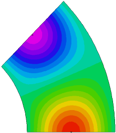
contour(u) on z=0.1 painted

contour(u) on z=0.5 painted

contour(u) on z=0.9 painted

end

3d_antiperiodic

3d_antiperiodic