<< Click to Display Table of Contents >> Navigation:  Sample Problems > Usage > Misc > spacetime1

{ SPACETIME1.PDE  

 

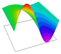
 This example illustrates the use of FlexPDE to solve an initial value problem

 of 1-D transient heatflow as a 2D boundary-value problem.  

 

 Here the spatial coordinate is represented by X, the time coordinate by Y,

 and the temperature by u(x,y).

 

 With these symbols, the transient heatflow equation is:  

       dy(u) = D*dxx(u),  

 where D is the diffusivity, given by  

       D = K/s*rho,  

       K       is the conductivity,

       s       is the specific heat,

 and   rho     is the density.

 

 The problem domain is taken to be the unit square.

 

 We specify the initial value of u(x,0) along y=0, as well as the time history

 along the sides x=0 and x=1.

 

 The value of u is thus assigned everywhere on the boundary except

 along the segment y=1, 0<x<1.  Along that boundary, we use the

 natural boundary condition,  

       natural(u) = 0,  

 since this corresponds to the application of no boundary sources on this

 boundary segment and hence implies a free segment.  This builds in the

 assumption that y = 1 (and hence t = 1) is sufficiently large for steady

 state to have been reached. [Note that since the only y-derivative term is

 first order, the default procedure of FlexPDE does not integrate this term

 by parts, and the Natural(u) BC does not correspond to a surface flux,

 functioning only as a source or sink.]

 

 This problem can be solved analytically, so we can plot the deviation

 of the FlexPDE solution from the exact answer.

 

}  

 

title "1-D Transient Heatflow as a Boundary-Value problem"  

select  

    alias(x) "distance"  

    alias(y) "time"  

 

variables  

    u  

 

definitions  

    diffusivity = 0.06    { pick a diffusivity that gives a nice graph }  

    frequency = 2         { frequency of initial sinusoid }  

    fpi = frequency*pi

  ut0 = sin(fpi*x)     { define initial distribution of temperature }  

    u0 = exp(-fpi^2 *diffusivity*y)*ut0   { define exact solution }  

 

Initial values  

    u = ut0              { initialize all time to t=0 value }  

 

equations  

    U: dy(u) = diffusivity*dxx(u) { define the heatflow equation }