<< Click to Display Table of Contents >> Navigation:  User Guide > Some Common Variations > Eigenvalues and Modal Analysis

FlexPDE can also compute the eigenvalues and eigenfunctions of a PDE system.

Consider the homogeneous time-dependent heat equation as in our example above,

together with homogeneous boundary conditions  

and/or

on the boundary.

 

If we wish to solve for steady oscillatory solutions to this equation, we may assert

 

The PDE then becomes

       

The values of and for which this equation has nontrivial solutions are known as the eigenvalues and eigenfunctions of the system, respectively.  All steady oscillatory solutions to the PDE can be made up of combinations of the various eigenfunctions, together with a particular solution that satisfies any non-homogeneous boundary conditions.

Two modifications are necessary to our basic steady-state script for the sample problem to cause FlexPDE to solve the eigenvalue problem.

•A value must be given to the MODES parameter in the SELECT section.  This number determines the number of distinct values of that will be calculated.  The values reported will be those with lowest magnitude.

•The equation must be written using the reserved name LAMBDA for the eigenvalue.

•The equation should be written so that values of LAMBDA are positive, or problems with the ordering during solution will result.  The full descriptor for the eigenvalue problem is then:

 

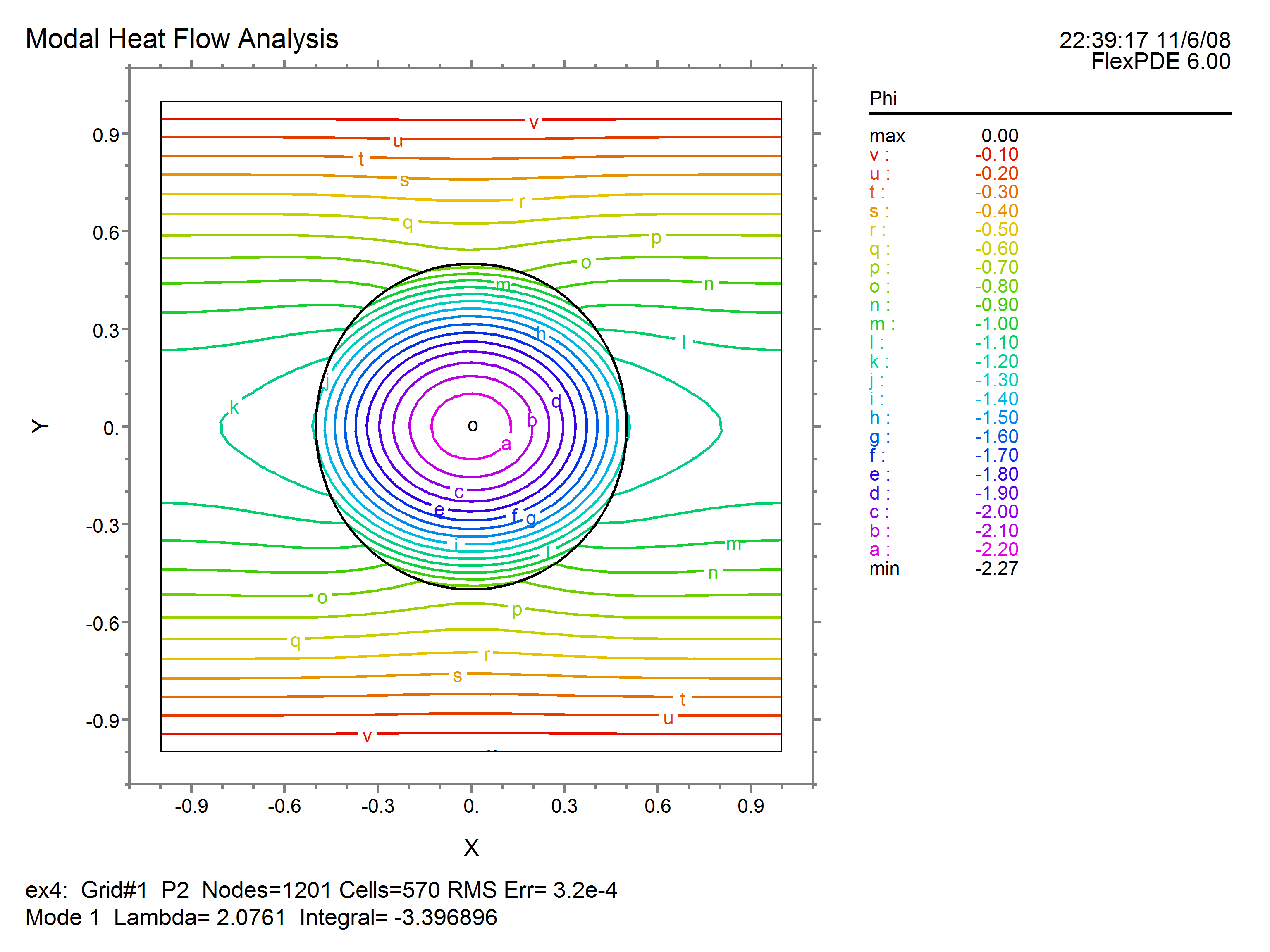
TITLE 'Modal Heat Flow Analysis'

SELECT

modes=4

VARIABLES

Phi                { the temperature }

DEFINITIONS

K = 1                { default conductivity }

R = 0.5        { blob radius }

EQUATIONS

Div(k*grad(Phi)) + LAMBDA*Phi = 0

BOUNDARIES

REGION 1 'box'

START(-1,-1)

VALUE(Phi)=0        LINE TO (1,-1)

NATURAL(Phi)=0        LINE TO (1,1)

VALUE(Phi)=0        LINE TO (-1,1)

NATURAL(Phi)=0        LINE TO CLOSE

REGION 2        'blob'        { the embedded blob }

k = 0.2                { This value makes more interesting pictures }

START 'ring' (R,0)

ARC(CENTER=0,0) ANGLE=360 TO CLOSE

PLOTS

CONTOUR(Phi)

VECTOR(-k*grad(Phi))

ELEVATION(Phi) FROM (0,-1) to (0,1)

ELEVATION(Normal(-k*grad(Phi))) ON 'ring'

END

 

The solution presented by FlexPDE will have the following characteristics:

•The full set of PLOTS will be produced for each of the requested modes.

•An additional plot page will be produced listing the eigenvalues.

•The mode number and eigenvalue will be reported on each plot.

•LAMBDA is available as a defined name for use in arithmetic expressions.

 
The first two contours are as follows: