| Author | Message | ||
Olivier Lami (ol9245) New member Username: ol9245 Post Number: 1 Registered: 04-2005 |
Hi all, I want to solve the following equations: 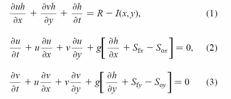 u and v are the flow velocity avove a free surface. The input data is the surface slope Sox and Soy, which are to be read in a file (grid with 10-cm cells). Thanks for helping | ||
Robert G. Nelson (rgnelson) Moderator Username: rgnelson Post Number: 348 Registered: 06-2003 |
The TABLE input command can be used to read tabular data of one, two or three dimensions. See TABLE in the Help Index. Incidentally, you will probably need to add some artificial diffusion to your equations to stabilize the solution. Your equations as written can support discontinuities in the direction normal to the flow paths, which is not handled well by the integral techniques of the finite element method. See the Technical Note "Smoothing Operators in PDEs". Try using a diffusivity on the order of D*c, where D is a "smearing" distance and c is an estimate of the magnitude of the velocities. | ||
Olivier Lami (ol9245) New member Username: ol9245 Post Number: 2 Registered: 04-2005 |
Hi, Thanks for helping. I tried TABLE. It Works fine. I am now trying to solve a steady state version of the equations above. R is rainfall I is Infiltration u and v are velocity I assume R-I = constant, and time-derivatives of h, u and v = 0. I wrote this this way and I got a bas message "An equation has collapsed to 0=0. An internal processing error has occurred Please contact PDE Solution Inc. bla bla bla" : variables H { depth } u { vx } v { vy } definitions Z = splinetable("my_elevation_file.dat") a = 2 {half width, m} b = 5 {half length, m} rain = 0.0000138888888888889 {m.s-1} f = 2 {darcy-weiback friction factor for bare sand} g = 9.81 Sfx = f*u*u/8/g/H Sfy = f*v*v/8/g/H Qx = u*H Qy = v*H Sox = dx(Z) Soy = dy(Z) equations dx(Qx)+dy(Qy)=rain { full Saint-Venant Equation} {u*DX(u)+v*DY(u)+g*(DX(H)-Sox+Sfx) = 0 u*DX(v)+v*DY(v)+g*(DY(H)-Soy+Sfy) = 0} {kinematic wave simplification} u: Sox=Sfx v: Soy=Sfy Boundaries region 1 start(-a,-b) load(v)=0 line to (a,-b) value(u)=0 line to (a,b) value(v)=0 line to (-a,b) value(u)=0 line to finish | ||
Robert G. Nelson (rgnelson) Moderator Username: rgnelson Post Number: 350 Registered: 06-2003 |
Unless otherwise instructed, FlexPDE initializes all variables to zero. If you plug zeroes into your original equations, you get the same thing as you have manually done in your "simplified" equations. So you have merely made explicit the condition that was implicit in the original. In the documentation relating to nonlinear equations, we say that FlexPDE uses Newton's method to solve nonlinear systems, and that a reasonable estimate of the solution is sometimes crucial to achieving a solution. Zero is not a reasonable estimate. Your equation is not a PDE, but merely an algebraic equation x^2=c Try solving F=x^2-c=0 by Newton's method: F'*delta(x) = -F or 0*delta(x) = c This is what FlexPDE means when it says that an equation has collapsed to 0=0. Probably it should say an equation has collapsed to 0=constant. Would this help? You must provide a reasonable guess for the solution. You would also probably do better to pose this problem in terms of a velocity potential, since first-order systems are somewhat intransigent in finite element methods. |