| Author | Message | |||||
Victor Bense (indiana) Member Username: indiana Post Number: 7 Registered: 01-2005 |
I would like to use SWAGE functions to avoid discontinutities. However, is there a way I can use muiltiple SWAGE commands for one variable. I try to capture something like the following in a SWAGE routine: Cb = if Temp > 0 then cf*rhof else if Temp < -2 then ci*rhoi else if Temp >= -2 and Temp <= 0 then ((1.0-f)*ci*rhoi+ f*cf*rhof)+ ls*rhof*(1.0-f)/40 else 1e10 How would that work? thanks, Victor | |||||
Victor Bense (indiana) Member Username: indiana Post Number: 8 Registered: 01-2005 |
OK, I partly fixed my problem by using a normal distribution over that interval. See the attached script. This is describing a melting permafrost layer. I implemented a very high heat capacity to overcome around the melting temperature (0 Celsius) which is now implemetned using that normal distribution as: cb_rest = if Temp > .2 then cf*rhof else if Temp < -.2 then ci*rhoi else if Temp >= -.2 and Temp <=.2 then ((1.0-f)*ci*rhoi+ f*cf*rhof) else 1e10 sigma=.25 Cb=0.03*rhof*ls*((1/(sigma*(2*pi)^.5)) *exp((-(Temp)^2)/(2*sigma^2)))+cb_rest Now the following problems remains. The peak of the normal distribution has to be higher than it is now. I should get rid of that factor 0.03. The script as it is runs fine, making the peak higher introduces numerical troubles. Is there a way around this? thanks again, Victor
| |||||
Robert G. Nelson (rgnelson) Moderator Username: rgnelson Post Number: 497 Registered: 06-2003 |
Normally, the way to proceed with this kind of thing would be to plot everything you can think of at every timestep, and look for something going strange. But I did this on this problem (melting1.pde), and nothing looked amiss. Yet the time integration was getting into trouble. Strange. On a hunch, I pulled Cb out of the time derivative, and it seems to run smoothly (melting2.pde). So apparently the time derivative of Cb is nasty, and is interfering with orderly integration. [Notice that dt(k*u)=k*dt(u)+u*dt(k). FlexPDE will do this expansion if k is time varying.] This modification alters the conservation properties somewhat. If this is a problem, a smaller TERRLIM might help, or making Cb a variable and manually expanding the time derivative. Incidentally, you can treate SWAGE() like any other mathematical function, multiply them, add them or nest them to achieve what you want.
| |||||
Victor Bense (indiana) Member Username: indiana Post Number: 9 Registered: 01-2005 |
Thank you for your help. I made some modifications but is still not behaving. I split the equation manually (melting3) which seems to slightly improve it as well I lowered TERRLIM significantly which also helps but doesnt solve the problem either. I am slightly confused on how to convert the functional relationship between Cb and Temp into a PDE and use that to stabilize things. Could you give an example of how to do that? thanks again, Victor
| |||||
Robert G. Nelson (rgnelson) Moderator Username: rgnelson Post Number: 498 Registered: 06-2003 |
Let me rephrase my previous statement. I believe the trouble in this problem is due to violent behavior of the time derivative of Cb, and I suggest that you take it outside the time derivative as I have done in the previously posted "Melting2.pde". If you are worried that this compromises accuracy, set TERRLIM smaller. I showed the derivative expansion merely to point out that FlexPDE will be computing the time derivative of Cb if it is left inside. Manually expanding the derivative does nothing that FlexPDE is not already doing. I tried making Cb a variable, and this does not help, because there are interpolation difficulties in adequately modeling the violent excursions. | |||||
Victor Bense (indiana) Member Username: indiana Post Number: 10 Registered: 01-2005 |
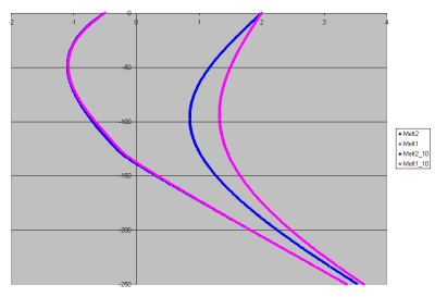
I compared the results of two runs puttingback in that factor 0.03 in the equation for Cb and using first "melting3": temp: (n*cb+(1-n)*rhos*cs)*dt(Temp)+div(q_heat)=0 and "melting4": temp: dt((n*cb+(1-n)*rhos*cs)*Temp)+div(q_heat)=0 In the first case I set TERRLIM=1e-6; XERRLIM=1e-4 In the second run I set ERRLIM=1e-4. As shown in Figure 1, the results are considerably different for later time (results shown for t=50 years and t=500 years). The blue line depicts the temperature profile for the case Cb is outside the time-derivative ("melting3") the pink-line is for when Cb is kept inside ("melting4"). Making TERRLIM smaller does not bring the two results closer together. Maybe the time-derivative is already having trouble in this case (with that 0.03 factor) when inside the time derivative ("melting4") and therefore gives a "wrong"-solution and the results for "melting3" are the actual correct ones? thanks, Victor
 | |||||
Victor Bense (indiana) Member Username: indiana Post Number: 11 Registered: 01-2005 |
Thanks for all of your help sofar. It is probably my inability to understand this. but clearly the two solutions are not entirely in agreement. So, should they? I mean is the difference a result of the difference in formulation of the equation. I see that when Cb is taken out of the time derivative its temporal variation (through temperature) is taken into account differently. I had the impression that you suggested that by setting a very low TERRLIM this discrepancy would be resolved (if I was worried about accuracy). Is that correct? However, that does not seem to happen. many thanks again, and I'll upload the files again including the transfer file.
| |||||
Robert G. Nelson (rgnelson) Moderator Username: rgnelson Post Number: 506 Registered: 06-2003 |
Clearly, using A*dt(B) in place of dt(A*B) is an approximation, and if A*B represents a conserved quantity, pulling the coefficient out degrades the conservation of the product. Depending on how active A is, this can be important or unimportant. In your case, I see that Temp is Quite well behaved, while the coefficient goes through a very sharply peaked transition, up by a factor of ten and back down by a factor of ten. The results you are comparing are the residue left over after adding and subtracting a very large quantity, and as such are subject to cancellation errors. The tracking of Cb must be very accurate or the upward and downward summations will not cancel. This accuracy requires both temporal and spatial resolution, since Cb will be interpolated in the mesh cells, and the variations over a single cell may be large. Since the activity of the coefficient is much more violent than that of the declared variable, the timestep and mesh-size control mechanisms that focus on Temp will be insufficient to guarantee accurate integration. The transition of Cb takes place in a window of +-0.2 around Temp=0, so one way to enforce tracking of Cb is to declare a FRONT at Temp=0 with a width of, say, 0.1. This will guarantee dense gridding during the crucial transitions of Temp. Also, there appears to be no X variation in your problem, so there is no reason to carry a lot of redundant cells in the x coordinate. You can narrow your mesh by a factor of 10 or 100 and save a lot of computation time. In the attached modification of Melting4.pde I have done these things, and it seems to run smoothly and efficiently.
|